How the simulation works

Simulating a solar tower.

A solar tower plant is a field of movable mirrors, each tracking the sun and reflecting it onto a receiver. How much energy actually lands on that receiver depends on where every mirror sits, how it is aimed, and how much light is lost on the way. Answering that question is what an optical ray tracer does.

The difficulty is that the answer is never needed once. Designing a field means asking it thousands of times, for thousands of candidate layouts, across a full year of sun positions. A ray tracer that is accurate but slow makes layout optimisation impossible. One that is fast but crude optimises the wrong field. Getting both at once is what this page is about. What we then do with that speed is the optimizer.

Where the light goes.

For a patch of mirror surface, the power reaching the receiver is the incoming solar irradiance reduced by a chain of efficiency factors:

P_int = I_DNI · A_cell ·η_cos · η_ref · η_aa ·η_sb · η_int

η_cos: Cosine effect. A tilted mirror presents a smaller area to the sun.
η_ref: Reflectivity. Not all light bounces off the mirror.
η_aa: Atmospheric attenuation. Light is scattered on the way to the tower.
η_sb: Shading and blocking. Neighbouring heliostats get in the way.
η_int: Intercept efficiency. How much of the reflected beam actually hits the receiver.

The first four are geometry and bookkeeping. The last, η_int, is where the hard part lives, and where ray tracers differ from one another.

Three kinds of uncertainty.

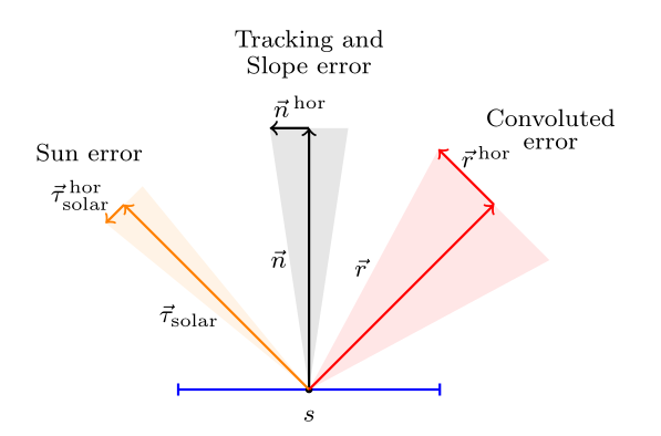
A reflected ray never goes exactly where geometry says it should, for three independent reasons:

Sun error. The sun is a disc, not a point, so rays arrive from a spread of directions.
Tracking error. A heliostat is aimed by two axes, and neither lands exactly on the intended orientation.
Slope error. Real mirror surfaces are not perfectly flat, and the deviation varies across the mirror.

Each is modelled as a Gaussian distribution. Combined, they give a single convoluted error cone around the ideal reflected ray. The width of that cone decides how much of the beam lands on the receiver instead of spilling past it.

Diagram showing the sun error on the incoming ray, the tracking and slope error on the mirror normal, and the resulting convoluted error cone on the reflected ray — Sun error perturbs the incoming ray. Tracking and slope error perturb the mirror normal. Together they give the convoluted error of the reflected ray.

Three ways to trace a ray.

Resolving that error cone is the whole game, and there are three ways to do it. They differ enormously in cost.

A single sampled ray leaving a mirror towards the receiver, drawn from a Gaussian distribution

Monte Carlo

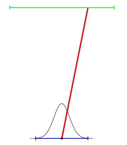
Draw one random ray from the error distribution and trace it. Accuracy improves with the square root of the ray count, so halving the noise costs four times the work.

A continuous cone of reflected light from a point on the mirror to the receiver

Convolution

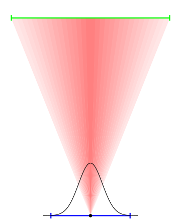
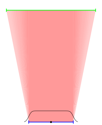
Stop sampling. Describe the error as a bivariate Gaussian and integrate it over the receiver directly. One evaluation replaces a cloud of random rays.

A wider integrated cone covering a whole mirror cell, with a flat-topped distribution at its base

Integrated convolution

Integrate across a whole mirror cell at once rather than a single point on it. This is the method introduced in our 2023 paper, and it is what makes the ray counts collapse.

What that buys you.

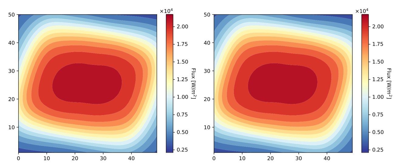
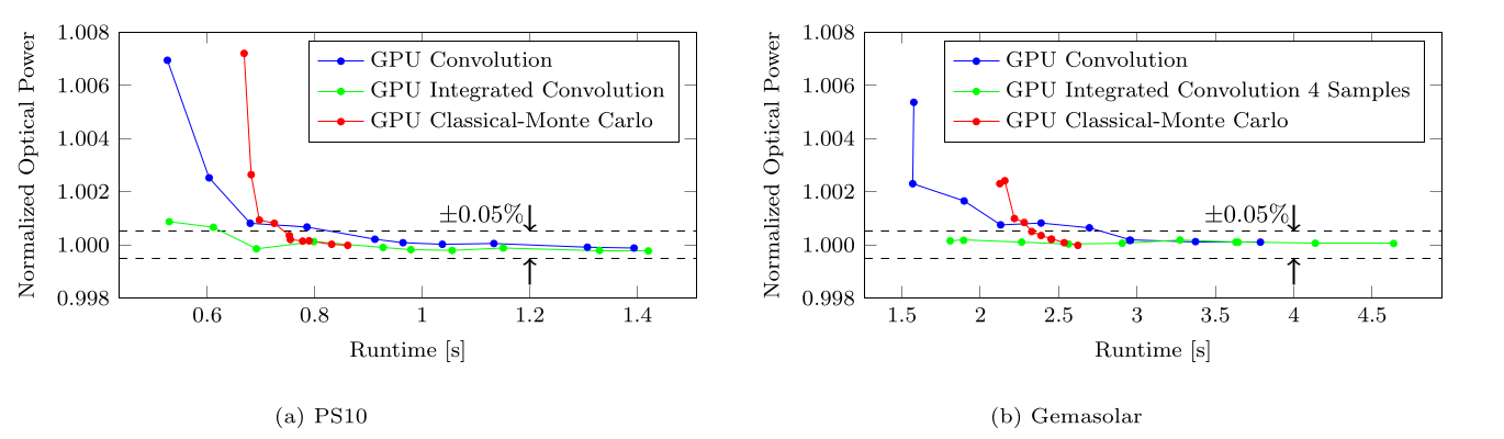
Two near-identical receiver flux maps, one computed with 7.5 billion Monte Carlo rays and one with 150 thousand rays using integrated convolution — The same receiver flux map on the PS10 test case. **Left:** Monte Carlo, 7.5 billion rays. **Right:** integrated convolution, 150 thousand rays. The relative difference stays below 1% in almost every cell.

Two charts plotting normalised optical power against runtime for GPU convolution, integrated convolution and Monte Carlo ray tracers, on PS10 and Gemasolar — Published GPU measurements: integrated convolution settles inside the ±0.05% accuracy band in roughly half the time the Monte Carlo tracer needs. Moving from CPU to GPU contributed a further factor of about 50.

Sampling a year.

Speeding up a single simulation is only half the saving. The other half is simulating fewer moments. Nobody runs all 8 760 hours of a year for every candidate layout, so annual simulation picks a few dozen representative ones. The common choice is every hour of the 21st of each month, which needs around 72 points.

We pick them somewhere else entirely. Rather than working in time, the plant efficiency is transformed into a celestial coordinate system. Seen in azimuth and elevation, a year traces an awkward dome that is hard to cover evenly. Seen in declination and hour angle, the same year fills a clean trapezoid, a shape you can map onto a unit square and cover with a small interpolation grid.

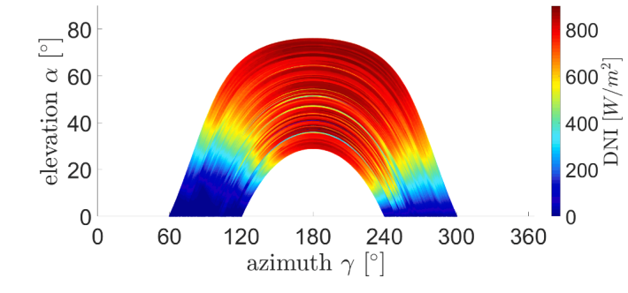
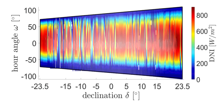
Annual sun path plotted against azimuth and elevation, forming a dome-shaped region coloured by solar irradiance — Horizontal coordinates: an awkward domain to sample.

The same annual sun path plotted against declination and hour angle, forming a trapezoidal region coloured by solar irradiance — Equatorial coordinates: a trapezoid you can grid.

Around 40 simulation points then reach 99.9% accuracy on both PS10 and Gemasolar. That is roughly three times faster than the standard approach, before the ray tracer itself has done anything clever.

Shading and blocking.

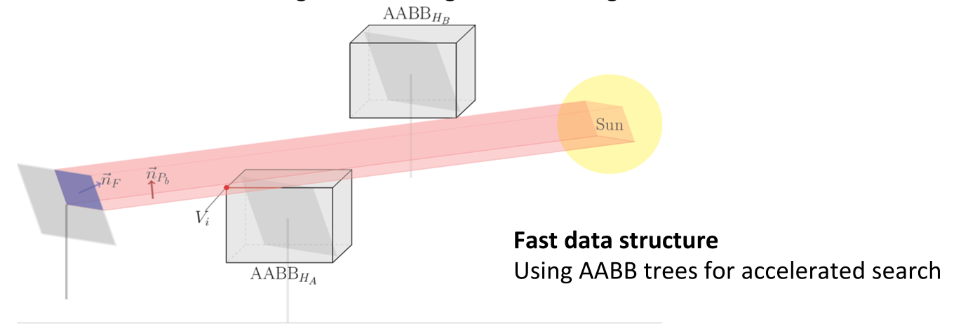
Before a ray is traced, you have to know which mirrors could get in its way. Candidates are narrowed with a bounding sphere test, then each heliostat facet is projected towards the sun and tested against the axis-aligned bounding boxes of the survivors. Those boxes live in an AABB tree, so search cost grows far more slowly than the field does. That is what keeps an 8 600-heliostat field tractable.

Diagram of a sun ray passing through the axis-aligned bounding boxes of two heliostats towards a mirror facet

Components we model.

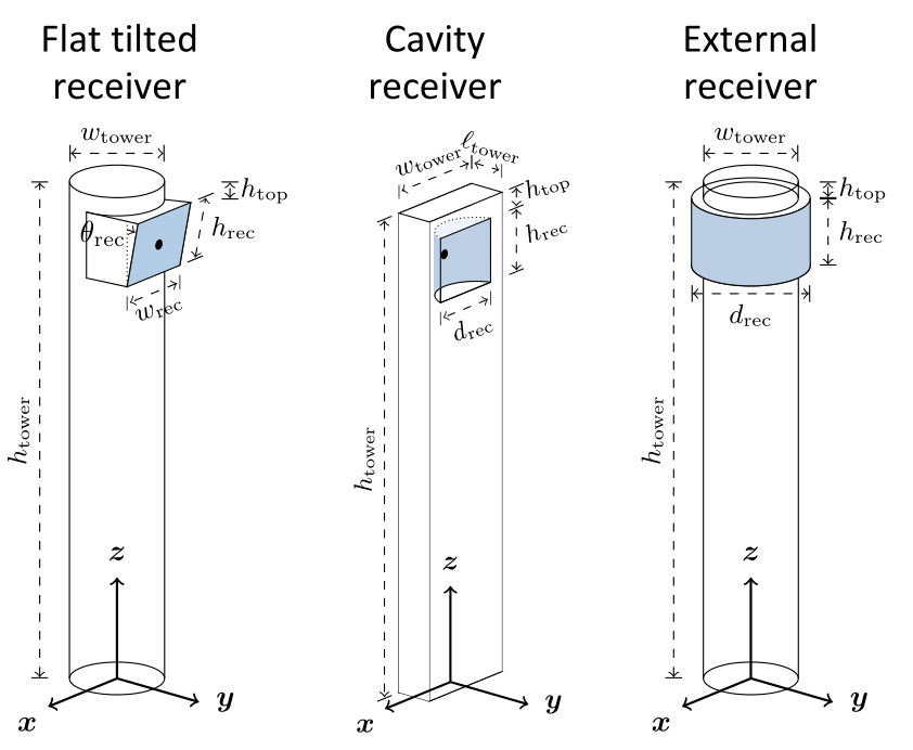
Heliostats support on-axis and off-axis canting using a parabolic function, and triangular facets. Three receiver types are modelled, each with its own geometry and aperture behaviour.

Geometry diagrams of a flat tilted receiver, a cavity receiver and an external receiver, each on a tower with labelled dimensions — Flat tilted, cavity and external receiver geometries.

Check it against your own tools.

SunFlower writes any project out as a SolTrace or Tonatiuh project, so you can reproduce our results in an independent Monte Carlo ray tracer on your own geometry. Output is an hourly efficiency breakdown: cosine, shading, blocking, soiling, reflectivity, atmospheric attenuation, spillage and total.

Request an API key

References.

F. Hövelmann, L. Aldenhoff, P. Richter. Analytic ray tracer on GPU for central receiver systems. Solar Energy, Volume 266, 112149 (2023). doi.org/10.1016/j.solener.2023.112149
P. Richter, J. Tinnes, L. Aldenhoff. Accurate interpolation methods for the annual simulation of solar central receiver systems using celestial coordinate system. Solar Energy, Volume 213, pp. 328–338 (2021). doi.org/10.1016/j.solener.2020.10.087

The equation, the error diagram, the method illustrations and the results figures are taken from the first paper. The annual sun path figures come from the second.