Designing the field.
A heliostat field is laid out once and then runs for twenty-five years. That layout fixes how much the plant will ever produce, and there is no fixing it later. Nobody can place 8 600 mirrors by hand, and every mirror you add shades and blocks its neighbours, so the positions cannot be chosen independently.
This is the part of the job that makes money, and it is why the simulator has to be fast. Finding a good layout means evaluating thousands of candidate fields across a full year. Every second saved in simulation is multiplied thousands of times over here.
What it found.
The honest test of an optimizer is whether it beats a field that real engineers already designed and built. We ran it against two: the PS10 and the Gemasolar, both in Seville.
- +1.8%PS10more annual optical power
than the layout as built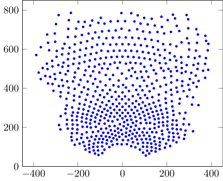
- +6.3%Gemasolarmore annual optical power
than the layout as built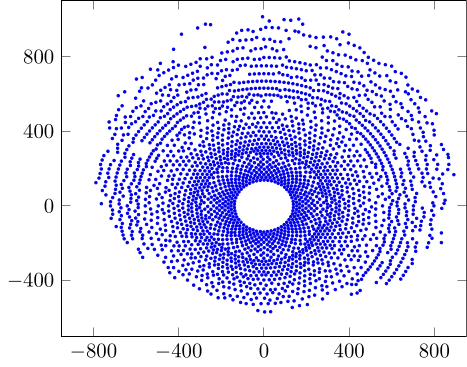
Same site, same hardware, same number of heliostats. Only the positions differ. Pattern optimisation alone reached +1.3% and +5.5%. The figures above add graph-based field growth.
Two ways to lay out a field.
Pattern optimisation
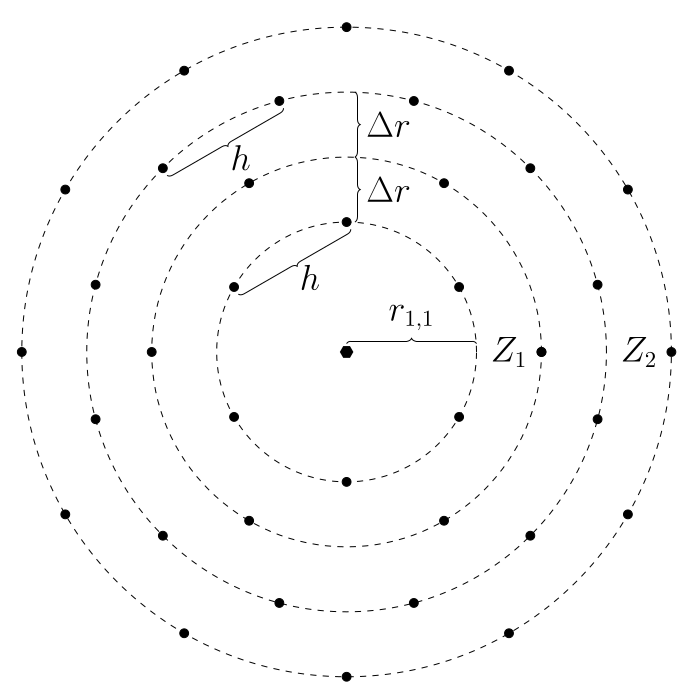
Heliostats are placed on a parameterised pattern, either cornfield, hexagon, radial staggered, rose or spiral, optionally stretched along an arbitrary axis. The optimizer searches the pattern's parameters, then a local search nudges individual mirrors.
This runs on the GPU. Accelerating the ray tracer, the annual integration and the heliostat collision detection together brought a full PS10 optimisation from three and a half hours down to 21 minutes.
Graph-based field growth
Rather than fitting a shape, this grows the field one mirror at a time. For every candidate position it evaluates exactly what that heliostat would collect and what it would cost the mirrors around it, tracked through a shading-and-blocking graph.
That exactness buys a guarantee patterns cannot give: no single heliostat can be moved to produce a better field.
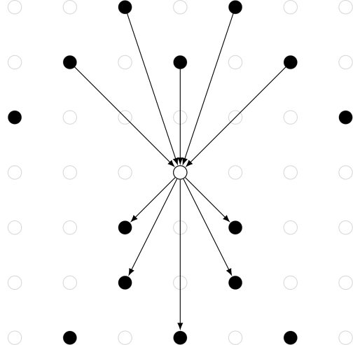
Field growth is the newer of the two and currently runs on the CPU, so on very large fields it takes longer than the GPU pattern route. Talk to us about which fits your case.
Put it to work on your site.
Optimisation is licensed as an add-on to the ray tracer. Send us your site, your weather file and your heliostat geometry, and we will show you what the layout is leaving on the table.
References.
- F. Hövelmann. Modeling and optimization of solar central receiver systems. Master's thesis, RWTH Aachen University (2022).
- P. Richter, D. Laukamp, L. Gerdes, M. Frank, E. Ábrahám. Heliostat field layout optimization with evolutionary algorithms. EPiC Series in Computing, Volume 41, pp. 240–252, GCAI (2016).
Figures on this page are taken from the first reference.
Get in touch.
Dr. Pascal Richter